Converting a dataset (combination of rows & columns ) into an Excel Table is one of the easiest & fastest ways to organize, filter, and analyze data. Instead of manually applying filters, borders, and formatting to a Dataset or Range, There is a simple Excel’s built-in Table feature, That does it all in a simple clicks. or else you can click a single keyboard shortcut. In this article, you’ll learn every method to create a table in Excel & how to name and format it, and it’s benefits.

Why to Use Tables in Excel Instead of a Normal Dataset?

Before going into deep, let’s see why it is required to Use Table instead of a Normal Dataset.

Table allows you to “Automatic filtering and sorting”,dropdown arrows appear on every column header instantly.

It has “Structured references“,formulas use column names instead of cell references, making them easier to read.

It allows you to “Auto-expanding range”,new rows or columns added at the edge of the table are automatically included.

It has “Built-in formatting feature“, which has banded rows, header styling, and totals row with one click.

“Easy to Analysis Data“, tables work seamlessly with PivotTables, charts, and with Power Query.

Table creation in excel is “Easy to use“. One simple short key converts your data set into Table in Excel. where you can filter and Analyse the data set.

It is easy to create and with a simple shortcut, with in a minute we convert the data set to Table.

Method 1: Create a Table Using the Keyboard Shortcut (Easiest & Fastest Way)

You can convert the Dataset to Table with easiest and Quickest way by just simply pressing one short key with just 2 fingers.

Lets see the below example: how to convert the Dataset into a Table. As shown in the below screenshot we have studentdata.

1. Select your dataset or place the cursor any where in range & press CTRL+ A, including the header row (e.g., student names and marks).

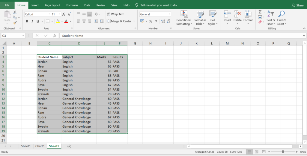
2. Press Ctrl + T on your keyboard or Press “CTRL” Key with One Finger and Letter with an another Finger “T”.

3. New pop window will open, Ensure that Data Range is correct.

4. Make sure that the table has headers and is checked if your data has column titles.

5.Click on “Ok” as shown below.

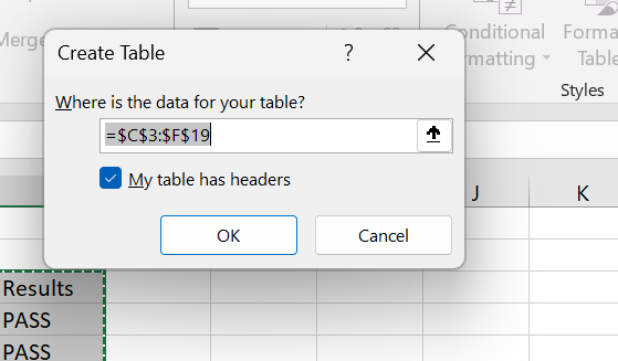
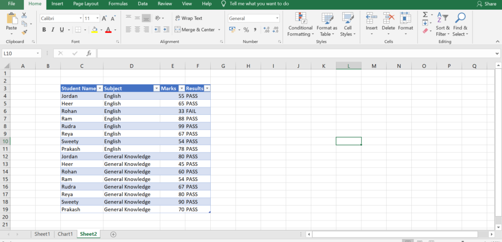
Your data range will instantly transform into a formatted Excel Table with filter arrows on each column header. click on Down Arrow to Filter the Results. Refer above Image

Select student name to get student wise output results

In our case we selected the student Rudra to get his marks, Refer below screen shots that how it can easily filter student information.

Conclusion: CTRL+T is the short key to convert any data set into Table in Excel within seconds. which reduces manual work and efforts.

Method 2: Create a Table from the Ribbon (Using Insert Tab)

Follow method 2 incase If you prefer using the ribbon instead of shortcuts:

1. Select any cell within your data range.

2. Go to the *Insert* tab.

3. Click *Table* in the Tables group.

4. Confirm the data range and header option, then click *OK*.

## Method 3: Create a Table with Specific Styling (Format as Table)

This method lets you pick a design while creating the table:

1. Select your data range.

2. Go to *Home → Format as Table*.

3. Choose a color/style from the gallery.

4. Confirm the range and headers, then click *OK*.

This is useful when you want a specific visual style applied immediately, rather than the default formatting.